How We Used JMH to Benchmark Our Microservices Pipeline
In a constant effort to improve metrics processing pipeline, LogicMonitor benchmarks the performance of the computation of complex datapoints. Learn more!
At LogicMonitor, we are continuously improving our platform with regards to performance and scalability. One of the key features of the LogicMonitor platform is the capability of post-processing the data returned by monitored systems using data not available in the raw output, i.e. complex datapoints.
As complex datapoints are computed by LogicMonitor itself after raw data collection, it is one of the most computationally intensive parts of LogicMonitor’s metrics processing pipeline. Thus, it is crucial that as we improve our metrics processing pipeline, we benchmark the performance of the computation of complex datapoints, so that we can perform data-driven capacity planning of our infrastructure and architecture as we scale.
LogicMonitor Microservice Technology Stack
LogicMonitor’s Metric Pipeline, where we built out a proof-of-concept of Quarkus in our environment, is deployed on the following technology stack:
Java 11 (corretto, cuz licenses)
Kafka (Managed in AWS MSK)
Kubernetes
Nginx (ingress controller within Kubernetes)
Why Did We Use JMH?
JMH (Java Microbenchmark Harness) is a library for writing benchmarks on the JVM, and it was developed as part of the OpenJDK project. It is a Java harness for building, running, and analyzing benchmarks of performance and throughput in many units, written in Java and other languages targeting the JVM. We chose JMH because it provides the following capabilities (this is not an exhaustive list):
We can configure the code being benchmarked to run a specified number of “warmup” iterations first before any measurement actually begins. This allows the JVM optimizations to take place before we are actually going to benchmark it.
We can configure the number of iterations the code will be run for benchmarking.
We can configure what we want to measure. Options available include throughput, average time, sample time, and single execution time.
We can configure JMH to allow garbage collection to take place during benchmark execution.
We can configure JMH to pass JVM runtime arguments during benchmark execution e.g. we can specify all different JVM memory options.
We can configure JMH to persist the report of the benchmark to file.
How Did We Benchmark the Computationally Intensive Code?
The first step for benchmarking computationally intensive code is to isolate the code so that it can be run by the benchmarking harness without the other dependencies factoring into the benchmarking results. To this end, we first refactored our code that does the computation of complex datapoints into its own method, such that it can be invoked in isolation without requiring any other components. This also had the additional benefit of modularizing our code and increasing its maintainability.
In order to run the benchmark, we used an integration of JMH version 1.23 with JUnit. First, we wrote a method that will invoke our complex datapoint computation with some test data. Then, we annotated this method with the @Benchmark annotation to let JMH know that we’d like this method to be benchmarked. Then, we actually configured the JMH benchmark runner with the configurations we wanted the benchmark to run with. This included:
How many warm-up iterations we wanted to use.
How many measurement iterations we wanted to use.
What do we actually want to measure? For our purpose, we set this to throughput.
We also had the option of specifying JVM memory arguments, but in this case, the code we were benchmarking was computationally intensive and not memory intensive, so we chose to forego that.
Finally, we annotated the JMH benchmark runner method with @Test, so that we could leverage the JUnit test runner to run and execute the JMH benchmark.
This is how our JMH benchmark runner method looks:
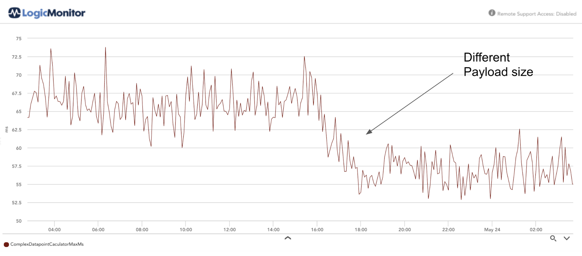
We ran the benchmark against different sizes of input data and recorded the throughput vs. size of input data. From the result of this, we were able to identify the computational capacity of individual nodes in our system, and from that, we were able to successfully plan for autoscaling our infrastructure for customers with computationally-intensive loads.
No. of complex datapoints per instance
Average Time (in ms)
10
2
15
3
20
5
25
7
32
11
Disclaimer: The views expressed on this blog are those of the author and do not necessarily reflect the views of LogicMonitor or its affiliates.